In “Mining sensor data, Part 1”, we continued our discussion on Sensor Data Analytics. I gave you a couple examples of how defects in a rotating machine might manifest in the machine vibration’s FFT signature. We briefly looked at the effects of motor shaft misalignment and bearing defects. In this post, I want to look at gears.

Figure 1: Gears Animation 1
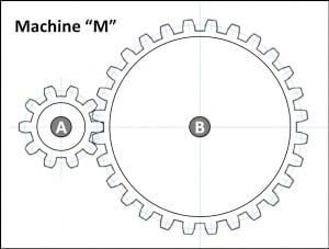
If we stop the animation of the two gear system animated in Figure 1, we can count the teeth on each gear. As shown in Figure 2, gear A has 10 teeth and gear B has 28.

Figure 2: Redrawn Gears have 10 and 28 teeth
Let’s say that gear A is driven at fA = 10 Hz (or revolutions/second). Then the GMF (Gear Mesh Frequency) will be 10 X 10 = 100 Hz. We can then take that 100 Hz and divide by 28 teeth/revolution for gear B and we have fB = 3.57 Hz. If we attach an accelerometer to Machine “M” and look at an FFT of the output, we can expect to see peaks at 10 Hz, 100 Hz and 3.57 Hz. We’ll often also see harmonics of those frequencies in the spectrum. Now suppose you have a fault on one of the teeth on gear B. This can cause spikes in the time domain at the gear B rotational frequency. These may manifest as +/- fB sidebands on the 100 Hz GMF peak in the frequency domain. Sometimes the FFT sidebands may be distorted by the physical transmission path between gears and sensor, and it may be easier to see the defect in the time domain.
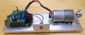
We have a relationship with the Arizona State University Sensor, Signal and Information Processing (SenSIP) Center in Tempe, Arizona. We’ve been sponsoring a project with SenSIP to explore how we might simplify machine learning for condition monitoring of machinery. I’ll touch more on machine learning in a later post. But right now I would like to expand the case above into a real world example. If you routinely read my blogs, you may recall a posting from last December entitled When prototyping, think “Maker”. That posting outlined the evolution of the test setup in Figure 3.

Figure 3: Third Generation Motor Vibration Test Setup
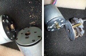
The motor in the setup includes a 4 gear gearbox. We gave one of these to Mr. Jongmin Lee, who is currently pursuing his PhD at ASU, and asked him to go crazy. He loaded the motor with a crude friction load, and ran it to failure (see Figure 4). Along the way, he took vibration data to determine if we could see differences over time.

Figure 4: After much abuse by Jongmin
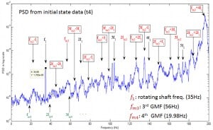
Figure 5 shows the power spectral density for measured vibrations early in the life of the motor. If you click on the figure, the expanded version will clearly show various frequency peaks that Jongmin has been able to relate to the motor, gear and gear mesh frequencies (with 4 gears, there are a lot of frequencies of interest).

Figure 5: Initial Power Spectral Density
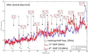
In Figure 6, he’s layered on the PSD as measured soon before motor failure. You can see some obvious changes in the spectrum.

Figure 6: Adding PSD shortly before motor failure
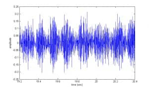
We can also look at raw data in the time domain. Looking at Figures 7 through 9, you can tell that something has changed over time. Jongmin tells me the envelope of the signal in Figure 7 is due to the friction load.

Figure 7: Raw vibration data early in the life of the motor
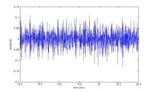
As the teeth of one of the gears (Figure 4) become worn, it causes some spikes and the time domain signal changes (Figure 8).

Figure 8: Mid-life raw vibration data
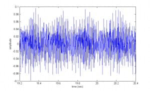
Finally the teeth are almost worn out, and the signal in Figure 9 is much less structured than the earlier plots.

Figure 9: Raw vibration data near end of life
The take-away from all of this is that you can often predict machine failure BEFORE it occurs, simply by looking at the vibration signature of the machine. By the way, the sensor used to take these measurements is the FXOS8700CQ2, which is a small (3 mm x 3 mm) consumer grade 6-axis device containing both accelerometer and magnetometer. It was configured to sample at 400 Hz for these examples.
My next posting will continue the “Mining Sensor Data” series, with a look at an everyday chaotic system you’ll find in your own kitchen.


